Particles in Glyph

Real-time GPU particle systems are the visualization paradigm SVG is worst at. Glyph can't do millions of particles at 60 fps — that's a different tool. But it can do the physics underneath them, deterministically, in one byte-stable SVG. Here's the best version, the animated variant, and the 4-step recipe to make either.

The output static · 144 trajectories

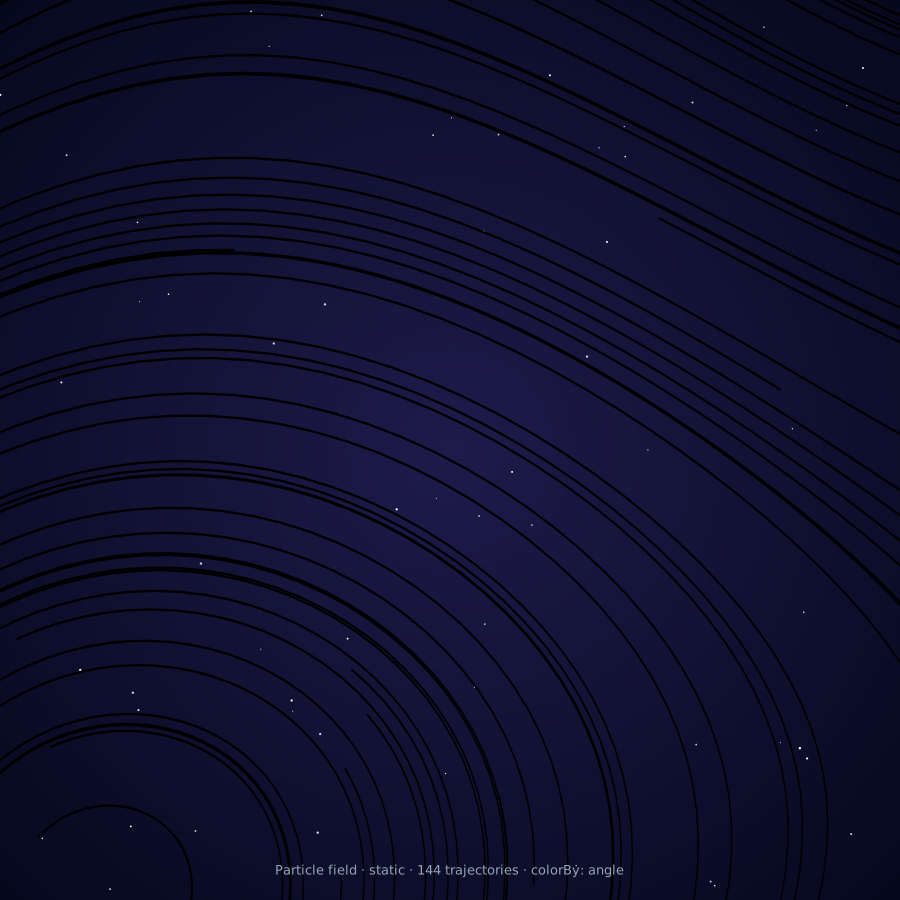
144 RK4-integrated trajectories. Color by local flow angle. One JSON spec → one SVG. Same bytes every time.

Same field, animated SMIL rotate-loop · 30 s per revolution

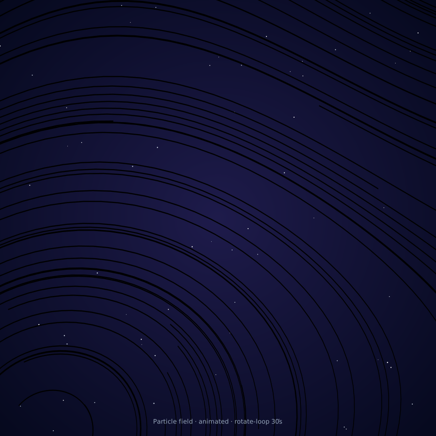
Open this in a browser to see it rotate. The streamlines stay fixed; the whole group spins around the center once per 30 seconds.

---

How to make it

Four steps. The whole spec fits on one page.

1. Define the vector field

   Write dx/dt and dy/dt as math expressions in two strings. Glyph's parser supports sin, cos, exp, sqrt, arithmetic, parentheses, and the variables x and y.

   // ABC-flavored field — two pairs of counter-rotating vortices
   "dxdt": "sin(2*y) + 0.4*cos(x)",
   "dydt": "-sin(2*x) + 0.4*sin(y)",
   "domain": { "x": [-3.14, 3.14], "y": [-3.14, 3.14] }

   Try other fields: "-y", "x" for pure rotation. Or "x*(1-x*x-y*y)", "y*(1-x*x-y*y)" for a limit-cycle attractor. Each one paints a different signature.

2. Pick your seed density

   The seeds block tells Glyph where to start each trajectory. grid seeds give an even sampling; bigger numbers = denser output.

   "seeds": { "kind": "grid", "rows": 12, "cols": 12 },
   "step": 0.04,        // RK4 step size (smaller = smoother)
   "maxSteps": 100      // trajectory length cap

   12×12 = 144 trajectories is a sweet spot for visual density without bloating the SVG.

3. Color the trails

   Three modes, each tells a different story:

   "colorBy": "step"      // rainbow from start to end of each trail
   "colorBy": "angle"     // color = local flow direction
   "colorBy": "magnitude" // color = local flow speed

   angle reads the cleanest at high seed counts. step is gorgeous but quadruples SVG size. magnitude highlights fast vs slow regions of the field.

4. Wrap it in compose, optionally animate

   Drop the chart into a compose scene with a dark background and (optionally) a SMIL rotate-loop on the chart child. The animation rotates the whole streamline group around its center.

   {
     "compose": {
       "viewBox": { "width": 900, "height": 900 },
       "theme": { "background": "#020617" },
       "children": [
         { "at": { "x": 50, "y": 50 },
           "size": { "w": 800, "h": 800 },
           "mark": "chart",
           "chart": { /* the streamline spec from steps 1–3 */ },
           "animation": {
             "kind": "rotate-loop",
             "periodMs": 30000,
             "direction": "ccw"
           }
         }
       ]
     }
   }

   Drop the animation block to get the static version. Keep it for the spinning-galaxy effect.

---

The full spec

If you want to copy + paste a working starting point, here's the entire spec (static variant). Run it through Glyph and you'll get the image at the top of this page.

{
  "compose": {
    "viewBox": { "width": 900, "height": 900 },
    "theme": { "background": "#020617" },
    "children": [
      { "at": { "x": 0, "y": 0 },
        "mark": "starfield",
        "starfield": { "count": 60, "seed": 13,
                       "region": { "x": 0, "y": 0, "w": 900, "h": 900 } } },
      { "at": { "x": 50, "y": 50 },
        "size": { "w": 800, "h": 800 },
        "mark": "chart",
        "chart": {
          "version": "glyph/0.1",
          "data": { "source": "inline:particles" },
          "layers": [{
            "mark": "streamline",
            "encoding": {
              "x": { "field": "x", "type": "quantitative",
                    "scale": { "domain": [-3.14, 3.14] } },
              "y": { "field": "y", "type": "quantitative",
                    "scale": { "domain": [-3.14, 3.14] } }
            },
            "streamline": {
              "dxdt": "sin(2*y) + 0.4*cos(x)",
              "dydt": "-sin(2*x) + 0.4*sin(y)",
              "seeds": { "kind": "grid", "rows": 12, "cols": 12 },
              "step": 0.04,
              "maxSteps": 100,
              "domain": { "x": [-3.14, 3.14],
                          "y": [-3.14, 3.14] },
              "colorBy": "angle"
            }
          }]
        }
      }
    ]
  }
}

Save as particles.json and run glyph render particles.json. Done.